St. Petersburg paradox
In economics, the St. Petersburg paradox is a paradox related to probability theory and decision theory. It is based on a particular (theoretical) lottery game (sometimes called St. Petersburg Lottery) that leads to a random variable with infinite expected value, i.e., infinite expected payoff, but would nevertheless be considered to be worth only a very small amount of money. The St. Petersburg paradox is a classical situation where a naïve decision criterion (which takes only the expected value into account) would recommend a course of action that no (real) rational person would be willing to take. The paradox can be resolved when the decision model is refined via the notion of marginal utility (and it is one origin of notions of utility functions and of marginal utility), by taking into account the finite resources of the participants, or by noting that one simply cannot buy that which is not sold (and that sellers would not produce a lottery whose expected loss to them were unacceptable).
The paradox is named from Daniel Bernoulli's presentation of the problem and his solution, published in 1738 in the Commentaries of the Imperial Academy of Science of Saint Petersburg (Bernoulli 1738). However, the problem was invented by Daniel's cousin Nicolas Bernoulli who first stated it in a letter to Pierre Raymond de Montmort of 9 September 1713 (de Montmort 1713).
Contents |
The paradox
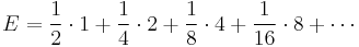
Consider the following game of chance: you pay a fixed fee to enter and then a fair coin is tossed repeatedly until a tail appears, ending the game. The pot starts at 1 dollar and is doubled every time a head appears. You win whatever is in the pot after the game ends. Thus you win 1 dollar if a tail appears on the first toss, 2 dollars if a head appears on the first toss and a tail on the second, 4 dollars if a head appears on the first two tosses and a tail on the third, 8 dollars if a head appears on the first three tosses and a tail on the fourth, etc. In short, you win 2k−1 dollars if the coin is tossed k times until the first tail appears.
What would be a fair price to pay for entering the game? To answer this we need to consider what would be the average payout: With probability 1/2, you win 1 dollar; with probability 1/4 you win 2 dollars; with probability 1/8 you win 4 dollars etc. The expected value is thus
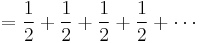
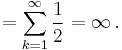
This sum diverges to infinity, and so the expected win for the player of this game, at least in its idealized form, in which the casino has unlimited resources, is an infinite amount of money. This means that the player should almost surely come out ahead in the long run, no matter how much he pays to enter; while a large payoff comes along very rarely, when it eventually does it will typically be far more than the amount of money that he has already paid to play. According to the usual treatment of deciding when it is advantageous and therefore rational to play, one should therefore play the game at any price if offered the opportunity. Yet, in published descriptions of the paradox, e.g., (Martin 2004), many people expressed disbelief in the result. Martin quotes Ian Hacking as saying "few of us would pay even $25 to enter such a game" and says most commentators would agree.
Solutions of the paradox
There are different approaches for solving the paradox.
Expected utility theory
The classical resolution of the paradox involved the explicit introduction of a utility function, an expected utility hypothesis, and the presumption of diminishing marginal utility of money.
In Daniel Bernoulli's own words:
- The determination of the value of an item must not be based on the price, but rather on the utility it yields…. There is no doubt that a gain of one thousand ducats is more significant to the pauper than to a rich man though both gain the same amount.
A common utility model, suggested by Bernoulli himself, is the logarithmic function u(w) = ln(w) (known as “log utility”). It is a function of the gambler’s total wealth w, and the concept of diminishing marginal utility of money is built into it. By the expected utility hypothesis, expected utilities can be calculated the same way expected values are. For each possible event, the change in utility ln(wealth after the event) - ln(wealth before the event) will be weighted by the probability of that event occurring. Let c be the cost charged to enter the game. The expected utility of the lottery now converges to a finite value:
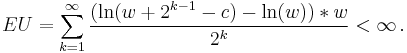
This formula gives an implicit relationship between the gambler's wealth and how much he should be willing to pay to play (specifically, any c that gives a positive expected utility). For example, with log utility a millionaire should be willing to pay up to $10.94, a person with $1000 should pay up to $5.94, a person with $2 should pay up to $2, and a person with $0.60 should borrow $0.87 and pay up to $1.47.
Before Daniel Bernoulli published, in 1728, another Swiss mathematician, Gabriel Cramer, had already found parts of this idea (also motivated by the St. Petersburg Paradox) in stating that
- the mathematicians estimate money in proportion to its quantity, and men of good sense in proportion to the usage that they may make of it.
He demonstrated in a letter to Nicolas Bernoulli [1] that a square root function describing the diminishing marginal benefit of gains can resolve the problem. However, unlike Daniel Bernoulli, he did not consider the total wealth of a person, but only the gain by the lottery.
This solution by Cramer and Bernoulli, however, is not yet completely satisfying, since the lottery can easily be changed in a way such that the paradox reappears: To this aim, we just need to change the game so that it gives the (even larger) payoff  . Again, the game should be worth an infinite amount. More generally, one can find a lottery that allows for a variant of the St. Petersburg paradox for every unbounded utility function, as was first pointed out by (Menger 1934).
There are basically two ways of solving this generalized paradox, which is sometimes called the Super St. Petersburg paradox:
- We can take into account that a casino would only offer lotteries with a finite expected value. Under this restriction, it has been proved that the St. Petersburg paradox disappears as long as the utility function is concave, which translates into the assumption that people are (at least for high stakes) risk averse [Compare (Arrow 1974)].
- We can assume that the utility function has an upper bound. Cramer had, in fact, also suggested a simple bounding under which all sums of money beyond some point would have equal utility (id est that the marginal utility of money would go to zero) (Bernoulli 1738), but a utility function need not become constant beyond some point to be bounded; for example the function
 is bounded above by 1, yet strictly increasing.
Recently, expected utility theory has been extended to arrive at more behavioral decision models. In some of these new theories, as in cumulative prospect theory, the St. Petersburg paradox again appears in certain cases, even when the utility function is concave, but not if it is bounded (Rieger & Wang 2006).
Probability weighting
Nicolas Bernoulli himself proposed an alternative idea for solving the paradox. He conjectured that people will neglect unlikely events (de Montmort 1713). Since in the St. Petersburg lottery only unlikely events yield the high prizes that lead to an infinite expected value, this could resolve the paradox. The idea of probability weighting resurfaced much later in the work on prospect theory by Daniel Kahneman and Amos Tversky. However, their experiments indicated that, very much to the contrary, people tend to overweight small probability events. Therefore the proposed solution by Nicolas Bernoulli is nowadays not considered to be satisfactory.
Rejection of mathematical expectation
Various authors, including Jean le Rond d'Alembert and John Maynard Keynes, have rejected maximization of expectation (even of utility) as a proper rule of conduct. Keynes, in particular, insisted that the relative risk of an alternative could be sufficiently high to reject it even were its expectation enormous.
One cannot buy what is not sold
Some economists resolve the paradox by arguing that, even if an entity had infinite resources, the game would never be offered. If the lottery represents an infinite expected gain to the player, then it also represents an infinite expected loss to the host. No one could be observed paying to play the game because it would never be offered. As Paul Samuelson describes the argument:
- Paul will never be willing to give as much as Peter will demand for such a contract; and hence the indicated activity will take place at the equilibrium level of zero intensity. (Samuelson 1960)
Finite St. Petersburg lotteries
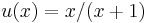
The classical St. Petersburg lottery assumes that the casino has infinite resources. This assumption is often criticized as unrealistic, particularly in connection with the paradox, which involves the reactions of ordinary people to the lottery. Of course, the resources of an actual casino (or any other potential backer of the lottery) are finite. More importantly, the expected value of the lottery only grows logarithmically with the resources of the casino. As a result, the expected value of the lottery, even when played against a casino with the largest resources realistically conceivable, is quite modest. If the total resources (or total maximum jackpot) of the casino are W dollars, then L = 1 + floor(log2(W)) is the maximum number of times the casino can play before it no longer covers the next bet. The expected value E of the lottery then becomes:
The following table shows the expected value E of the game with various potential bankers and their bankroll W (with the assumption that if you win more than the bankroll you will be paid what the bank has):
| Banker | Bankroll | Expected value of lottery |
| Friendly game | $100 | $4.28 |
| Millionaire | $1,000,000 | $10.95 |
| Billionaire | $1,000,000,000 | $15.93 |
| Bill Gates (2008) | $58,000,000,000 | $18.84 |
| U.S. GDP (2007) | $13.8 trillion | $22.78 |
| World GDP (2007) | $54.3 trillion | $23.77 |
| Googolaire | $10100 | $166.50 |
Notes: The estimated net worth of Bill Gates is from Forbes. The GDP data are as estimated for 2007 by the International Monetary Fund, where one trillion dollars equals $1012 (one million times one million dollars). A “googolaire” is a hypothetical person worth a googol dollars ($10100).
A rational person might not find the lottery worth even the modest amounts in the above table, suggesting that the naive decision model of the expected return causes essentially the same problems as for the infinite lottery. Even so, the possible discrepancy between theory and reality is far less dramatic.
The assumption of infinite resources can produce other apparent paradoxes in economics. See martingale (roulette system) and gambler's ruin.
Iterated St. Petersburg lottery
Players may assign a higher value to the game when the lottery is repeatedly played. This can be seen by simulating a typical series of lotteries and accumulating the returns; compare the illustration (right).
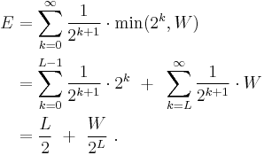
If the expected payout from playing the game once is E1, the expected average per-game payout from playing the game n times is:
Since E1 is infinite, En is infinite as well. Nevertheless, expressing En in this way shows that n, the number of times the game is played, makes a finite contribution to the average per-game payout. The actual average per-game payout obtained in a series of n games is unlikely to fall short of this finite contribution by a significant amount.
To see where the (1/2) log2 n contribution comes from, consider the case of n = 1,024. On average:
- 512 games will pay $1
- 256 games will pay $2
- 128 games will pay $4
- 64 games will pay $8
- 32 games will pay $16
- 16 games will pay $32
- 8 games will pay $64
- 4 games will pay $128
- 2 games will pay $256
- 1 game will pay $512
→ From here on it is equivalent to: 1 game will pay out 1,024 x E1
- (1/2) game will pay $1,024
- (1/4) game will pay $2,048
- etc.
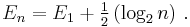
The collective average payout is therefore $5,120 (Until the arrow sign) + 1,024 x E1, and the per-game average payout is:
Because the finite contribution from n games is proportional to log2 n, doubling the number of games played leads to a $0.50 increase in the finite contribution. For example, if 2,048 games are played, the finite contribution is $5.50 rather than $5.
It follows that, in order to be reasonably confident of achieving target average per-game winnings of approximately W (where W > $1), we should play approximately 4W games. This will yield a finite contribution equal to W. Unfortunately, the number of games required to be confident of meeting even modest targets is astronomically high. $7 requires approximately 16,000 games, $10 requires approximately 1 million games, and $20 requires approximately 1 trillion games.
Further discussions
The St. Petersburg paradox and the theory of marginal utility have been highly disputed in the past. For a discussion from the point of view of a philosopher, see (Martin 2004).
See also
Works cited
- Arrow, Kenneth J. (February 1974). "The use of unbounded utility functions in expected-utility maximization: Response" (PDF). Quarterly Journal of Economics (The MIT Press) 88 (1): 136–138. doi:10.2307/1881800. JSTOR 1881800. Handle: RePEc:tpr:qjecon:v:88:y:1974:i:1:p:136-38. http://ideas.repec.org/a/tpr/qjecon/v88y1974i1p136-38.html.
- Bernoulli, Daniel; Originally published in 1738; translated by Dr. Lousie Sommer. (January 1954). "Exposition of a New Theory on the Measurement of Risk". Econometrica (The Econometric Society) 22 (1): 22–36. doi:10.2307/1909829. JSTOR 1909829. http://www.math.fau.edu/richman/Ideas/daniel.htm. Retrieved 2006-05-30.
- de Montmort, Pierre Remond (1713) (in (French)). Essay d'analyse sur les jeux de hazard [Essays on the analysis of games of chance] (Reprinted in 2006) (Second ed.). Providence, Rhode Island: American Mathematical Society. ISBN 978-0821837818. as translated and posted at Pulskamp, Richard J. "Correspondence of Nicolas Bernoulli concerning the St. Petersburg Game" (PDF (88 KB)). http://www.cs.xu.edu/math/Sources/Montmort/stpetersburg.pdf. Retrieved July 22, 2010.
- Martin, Robert (2004). "The St. Petersburg Paradox". In Edward N. Zalta. The Stanford Encyclopedia of Philosophy (Fall 2004 ed.). Stanford, California: Stanford University. ISSN 1095-5054. http://plato.stanford.edu/archives/fall2004/entries/paradox-stpetersburg/. Retrieved 2006-05-30.
- Menger, Karl (August 1934). "Das Unsicherheitsmoment in der Wertlehre Betrachtungen im Anschluß an das sogenannte Petersburger Spiel". Zeitschrift für Nationalökonomie 5 (4): 459–485. doi:10.1007/BF01311578. ISSN 0931-8658. (Paper) (Online).
- Rieger, Marc Oliver; Wang, Mei (August 2006). "Cumulative prospect theory and the St. Petersburg paradox". Economic Theory 28 (3): 665–679. doi:10.1007/s00199-005-0641-6. ISSN 0938-2259. (Paper) (Online). (Publicly accessible, older version.)
- Samuelson, Paul (January 1960). "The St. Petersburg Paradox as a Divergent Double Limit". International Economic Review (Blackwell Publishing) 1 (1): 31–37. doi:10.2307/2525406. JSTOR 2525406.
Bibliography
- Aumann, Robert J. (April 1977). "The St. Petersburg paradox: A discussion of some recent comments". Journal of Economic Theory 14 (2): 443–445. doi:10.1016/0022-0531(77)90143-0.
- Durand, David (September 1957). "Growth Stocks and the Petersburg Paradox". The Journal of Finance (American Finance Association) 12 (3): 348–363. doi:10.2307/2976852. JSTOR 2976852.
- "Bernoulli and the St. Petersburg Paradox". The History of Economic Thought. The New School for Social Research, New York. http://cepa.newschool.edu/het/essays/uncert/bernoulhyp.htm. Retrieved 2006-05-30.
- Haigh, John (1999). Taking Chances. Oxford,UK: Oxford University Press. pp. 330. ISBN 0-19-850291-9.(Chapter 4)
- Samuelson, Paul A. (March 1977). "St. Petersburg paradoxes: defanged, dissected, and historically described". Journal of Economic Literature 15 (1): 24–55.